Sunday, January 31, 2016

Reflecting on Lossyness and Evolving images

A few years ago I tried playing with trying to evolve images out of polygons.  After the post by Roger Alsing that started it all a number of people pondered whether or not it would be usable as a form of image compression.   I was doubtful but gave it a go anyway.  It turned out to be rather competitive at extremely high compression rates.   For my samples I compressed color 256x256 images down to 800-1200 bytes,  achieving quality levels better than many other compression methods.  Those are, however extremely high compression rates in the 0.1 to 0.15 bit-per-pixel range, and should be considered in that context.  For  example I managed to generate a 256x256 Lena image at 1024 bytes with 25psnr.

To get a perspective on where that lies, This paper has a number of graphs showing the rapid decline in quality as bits per pixel approaches zero. 
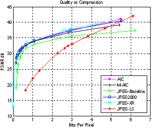
So that's where things stood when I last played with it.  I might be ready to have another go at it. 

Before I dive into it I felt I should write about some of the things that I learned from my previous experience.  Working with the evolver gave me plenty of things to ponder, and I think much of what I have learned came slowly to me during the intervening years as I thought about what it realy means.


Thinking about lossiness and expressiveness 

One of the things my experience helped me with was formalising what is essentialy the obvious idea behind the process of evolving pictures.  The ideal evolvable representation is a dataform which can express the widest range of images while maintaining a similarity between codes with minor differences.   The second aspect of that principle is easy to accommodate, a bitmap does almost exactly this.  A bitmap does a very poor job satisfying the first principle though because the range and difference required has to be considered in the space of everything that humans can perceive.

Here's an example to show the problem.

Spot the Difference.
A and B are one pixel different as are C and D


A single pixel change in the second pair of 64x64 images can be more easily perceived than the first because the image is simpler.   If you are considering each image to occupy a position in the space of human perceivable images you would say the distance between A and B is less than C and D.

The ideal image representation would be something where every codeable image formed evenly spaced points in the full field of humanly perceivable things.    That is ultimately the best that any lossy data compression can achieve.   Finding such a representation is difficult, if not impossible.   Even identifying what is perceivable is a difficult question.  At present, it is even a difficult task to evaluate just how perceptibly different two images are.  Stuctural Similarity (SSIM) is used over Peak Signal to Noise Ratio (PSNR) in many tests.   SSIM is still an extremely crude approximation of what happens during the interaction of the senses and the mind.   To make matters worse, given that our perceptions are also colored by our knowledge, learning more about perception can alter how we perceive things.

Consider this hypothetical idea,  If it were possible to calculate an evenly populated field all perceivable images you could compress any image down to any size with the best possible results.   If you could populate the field with 4 billion evenly spaced points the resulting images could be represented in 32 bits.  Such a compression rate would undoubtedly be extremely lossy, but from a pool of 4 billion distinct images it might get surprisingly close.   This idea is the essence of lossy compression.   Any lossy algorithm aims to produce data that satisfies that criteria.

If you mapped all bit combinations of data of a existing formats you would find points in the field of human perception with uneven spacing and clusters around certain zones.  This is because nobody has yet invented the perfect Image compression algorithm yet.  There is a good reason for that.  We have no idea of what the space of human perception is.  It's probably some many dimensional blob bulging in odd places.  Even if we knew this,  I'm not sure if there would be an accurate way of collecting data on a format short of trying every possible bit pattern.   Hopefully, people way smarter than I are working on these issues.

Even though the ideal is vastly beyond our current reach, it at least can serve as a guide towards what is the right direction.   Changes in data should produce perceivable differences,  but to evolve, small changes should also produce similar images.

In the context of rendering images out of polygons I used irregular hexagons with a bit to encode whether or not to round the edges and a few bits to indicate a blurred edge.  They were easy decisions because looking at other polygon evolvers,  triangles seemed to be insufficiently expressive and images frequently have gradients which are difficult to represent with hard edged objects.

Recently I looked at doing a form of the Image renderer using a GPU shader.   Instead of rendering a polygon and Gaussian blurring it,  my plan was to use distance fields.   When I used hexagons, the evolver managed to do some impressive tricks utilizing self intersecting shapes.  It turns out computing a distance field for a self intersecting hexagon is not as easy as it sounds.  While struggling with the problem, I had a small epiphany.  Two triangles that can combine in multiple ways might be even more expressive.  Here's where I ended up as a base gene.

   red,green,blue,alpha : uint6;
   a1,b1,c1 : {uint8,uint8} //triangle 1 clockwise filled anticlockwise outline.
   a2.b2.c2 : {uint8,uint8} //triangle 2 clockwise filled anticlockwise outline.
   falloff : uint5;
   combineOp : uint3;  // (or, smooth_or, subtract, union...  possibly more )

   Total: 16 bytes;


Here's what the shader can generate from six points.  This returns an alpha value which is combined with the RGBA of the 'gene'.  The combination mode would not be very changeable in a evolving image.  The points should be able to drift freely to make a large number of distinctly different looking shapes.  If the shapes do not intersect at all they take on the appearance of individual triangles.

You can see a version trying various falloff levels on shadertoy

Thinking about Collaborative Image Compression.

When I tried evolving polygon, it was fairly evident that it would not be competitive with compression methods that aim for PSNR values over 30.  The reason was obvious. at that level textures and patterns start becoming apparent which frequency based algorithms can utilize.  Evolved polygons are blissfully unaware of such matters.   This lead me to wonder about mixing methods.

Many a naive coder has had the brilliant idea to try and improve the compression rate of lossless compression by compressing a lossy image and a lossless error map.   After trying a JPEG+PNG  combination they find the combination of the two images is usually more than a PNG on its own.  I have seen a number of people do this, and I did it myself when I was much younger (although I did not use PNG due to it not being invented yet)

That this one way to do it does not work does not invalidate the entire method.  In fact PNG itself does a simple form of this internally.  The main distinction between PNG filters and storing a lossy image as a base is that the filter guesses the next pixel based upon what has already been encoded.  It frequently guesses wrong, but by guessing it doesn't have to store any additional data to make the guess in the first place.   Sometimes this can make things worse if the guesses are consistently wrong.  The corrections might compress less well than the original data would have.  Overall it tends to be a gain.

To take the step of encoding data to provide a base image is a more difficult task.   For every additional byte of data you add to the first stage, you must improve the final stage by more than a byte.  For lossy compression it becomes more unclear,  for every byte spent, you must gain more than a byte's 'worth'.   Since we are aiming for quality, the question is more to do with whether or not spending the byte early or spending it later results in the best image.

You may now see why this idea became of interest to me again after experimenting with the evolved images.    The broad strokes approach of the polygon renderer exhibits the sort of profile we would look for in a first stage.  It exhibits the most rapid gains towards the target image at the lowest bit-per-pixel rates.

The area that I would really like to explore is the idea of eliminating the concept of a first pass followed by a correction pass,  but to see if a dynamically collaborative process could be obtained.    Have a modular compression system where a compression algorithm module receives a working-image and an allocation of bytes and it tried to spend its bytes on encoding a modification to the working-image to better match the goal image.

The polygon evolver approach roughly resembles this mechanism already.  Each polygon is encoded into a number of bytes and is rendered on top of the existing image.   Polygons exist as 16 byte packets.  Adding a polygon (after evolution) results in a net gain in image quality.  

Extending this principle to multiple encoding methods has advantages and disadvantages. The advantages are obvious, using multiple techniques permits specialization . Specialization means the best performing technique can be chosen for image components. The main disadvantage is that specialization requires extra data to encode what method is chosen and where in the image that data applies.

In normal image compression some of the required information is implied by the format or context.  DCT compressed images like JPEG store blocks as (usually) 8x8 cells.  The same image could be encoded in a multi-algorithm image if it had a DCT module that handled a cell per data packet.  The resulting image would look the same but have a larger data size.  Every packet would have to encode data to say "This is a DCT cell at position x,y".   JPEG gets that data for free.  It's DCT because that's what JPEG does, and the position is "right after the last cell we decoded".

You could potentially squeeze that extra data into a small space, a data packet beginning  single zero bit could indicate a the same type as the previous.  Similarly if a DCT packet began with a zero it could indicate that it comes right after the previous cell in the picture.  That would mean our hypothetical all-DCT image might only gain an additional 2 bits per cell.   You wouldn't do that of course.  Enabling multiple encoding techniques then using a single one eliminates all of the advantages of the system.

Where this idea would work best is for mixing a few techniques together.  You may only end up with 5 DCT blocks in an image strategically placed in places where the polygonal method fails the worst.  Or perhaps a glyph encoder is a better solution where it encodes on the assumption that it is encoding a bi-level or alpha-mask image where set pixels are usually by other set pixels and clear pixels are usually by other clear pixels.

Generating images using all these methods together is an interesting challenge. but I think it might be doable. 


Before I dive into that part, I should first make a WebGL polygon shader evolver using my triangle pairs approach to hee how well it works.


Friday, January 1, 2016

A Little Calculator.

I'm trying out Cinnamon. It seems to be quite a nice environment, but I couldn't find a Calcuator that met my needs. This was the Calculator I found.
For me, it was too large and inflexible. I wanted something where I could type in complex expressions and easily do so while referring to the contents of another window.

My criteria were:
  • Small: So it does not obscure the information I am referring to for the calculation
  • Stay-on-top: So that when I click on a window to type in the result of the calculation, the calculator doesn't disappear
  • Draggable: So if it is in the way it can readily moved to another spot
  • Easy to summon and dismiss
  • Expressions can be typed in directly
  • Support for Hex and Binary
  • Recallable history
I have used a little Calculator on my Windows machine for years that has all of these properties. I couldn't find what I wanted there either, so I knocked together something in Delphi. It has been an extremely useful little thing that has come in handy for many years now (the .exe I still use has a creation date of 2003) . So I've only been using Cinnamon a couple of months now and I'm quite new to using Clutter, but here's what I have managed so far.
It's on GitHub

Tuesday, October 13, 2015

Hex Cellular Automata

I have a project that could use a massive field of fluid as a base. To do this I'm going to need to be able to do a decent speed fluid simulation, This is my first attempt at doing any sort of fluid at all. My previous post shows the various states that the cells can have. I managed to cobble together a decent JavaScript implementation.

This implements a 350x250 hex grid, The actual field size that I want to have will be much larger and will require GPU accelleration.

Thursday, October 8, 2015

Symmetry

I'm making a Cellular Automata on a hex grid. Before I actually write the code for the cells I had to write this visualisation to ensure I got the rules correct, The same rule should apply for all cells of the same structure regardless of orientation, so all rotations and flips get the same rule.

After writing this I'm fairly certain I would have screwed up the rules without it. Trying to detect mistakes from the behaviour of the rules would be nearly impossible I think.. Mouse over cells to see the matches.


Wednesday, September 30, 2015

Charged Particles

I wrote this little program while I waited for some SDKs to download. It's just a toy to play with the dynamics of charged particles. While not directly accurate to any real world physical model (not least because it is only 2D), it can demonstrate some principles of chemistry. The principles of molecules and chemical reactions can be seen as charged particles attract, assemble and react to the presence of new charges.


Left, Middle, and Right mouse buttons place particles of -1, random, +1 respectively

Use number keys 1-9 & 0 to place particles in a range of -1 to +1

Wednesday, September 16, 2015

Stack Machine generated Textures

This is something I made Just a few weeks ago. You feed it Strings and it gives you Textures, It's not an easy thing to use but I find it quite fun.  The goal was to provide the ability to include small textures inside code. 

The images are generated in a reverse polish notation stack expression.  The expression is calculated for every pixel in the image, with x and y indicating the current pixel location within the image.   The codes that stackie understands are:

     x : push x (x is in range 0...1)
     y : push y (y is in range 0...1)
     0...9 : push constant 0...9
     P : push PI

     d : duplicate top item on the stack
     : : swap top two items on the stack
     ; : swap top and third items on the stack

     s : sin
     c : cos
     q : sqrt
     ~ : abs
     ! : flip        1-a                  implemented as  push(1-pop())
     # : round to nearest integer
     ? : threshold  ( value<=0 becomes 0, value>0 becomes 1 ); 

     p : perlin noise (using top two stack values)
     w : wraparound perlin noise using three stack valuesx,y,size
     W : wraparound perlin noise using 4 stack values x,y,x_size, y_size

     a : atan2
     + : add
     - : subtract
     * : multiply
     / : divide
     ^ : pow        
     > : max        
     < : min        

While the final strings can look incomprehensible, writing a texture code is easier than it seems.  You can build it up by constructing simple pieces and mixing them together
x y
x and y make simple vertical and horizontal gradients.
x! y!
! inverts the value
xy* xy+2/
Multiply two gradients together, or add them together and divide by 2 for a simple average
xyp x8*y8*p1+2/
p generates perlin noise. For higher frequency noise multiply the x and y values by a scale factor


x9^ y9^
x9^ y9^ + x9^ y9^ + x!9^ y!9^ + +

By combining simple sequences together you can construct  more complex images.
x8* y3* p 1+ x9^ x!9^ + y! + +
x8* y3* p 1+ x9^ x!9^ + y! + - Palette xy!1+*
Have a play around with it in the iframe


Stackie is on github

Tuesday, September 15, 2015

8 bit machine

I have been making a 8 bit emulator for a non existent machine.   The specs of the machine are

Processor8-bit AVR
Intruction SetArduino Compatible
Program Memory128k (0000-FFFF x 16-bit)
RAM64k (0000-FFFF x 8-bit)
Display480x360 / 240/180


There is a 512x392 24bit FrameBuffer that exists as a necessity for rendering onto a canvas.  The CPU does not have direct access to the buffer and cannot read from it at all.

If I were writing an emulator that was closer to 8-bit machines of years past, There would be no framebuffer. In those days Pixels were all about timing. You coloured the pixel as the video beam went past. Video chips (or sometimes the CPU itself) had do construct the image line-by-line. Few systems had enough memory to hold a completed grid of pixels ready to go.

The transience of the display was also an advantage for those old machines. By changing the video hardware parameters during the screen update you can achieve a variety of effects. Display hardware that could show a limited number of sprites could have more appear on screen than there actually were, because you can shift them around after the video beam has passed in order to be seen by the beam a second time later down the screen. You could bend and colour things on the screen using similar so-called raster effects. What was an advantage for the old is however a disadvantage for the new. Emulators that strive for accurate emulation of old video hardware must put in a great deal of extra work to measure the timing and to generate an image from an emulated video beam on an emulated video display. Usually emulators will have to do this to fill a FrameBuffer image that will be placed on-screen by the operating system as a single bulk operation.

I decided to make the FrameBuffer a defined part of this emulator in order to reduce the workload of the emulator, It means the raster effects of old video displays will not be possible but in return there will be some advantages for the machine where it can construct a frame at a time instead of as a series of sequential pixels.

The FrameBuffer that the emulator uses is 802,816 bytes. In its raw form it would be cumbersome and slow for an 8 bit processor to write to. The CPU interface to the FrameBuffer aims to allow as much as possible for as little data and processing as possible.

There are 16 I/O ports associated with the video output ( Currently based at I/O port 0x20, may change ).

+ 0x00 pixelData_diaplayStart_L
+ 0x01 pixelData_displayStart_H16-bit address
+ 0x02 colorData_displayStart_L
+ 0x03 colorData_displayStart_H16-bit address
+ 0x04 pixeldata_increment
+ 0x05 colorData_increment
+ 0x06 pixelData_lineIncrementvalue << 3 to make 11-bits
+ 0x07 colorData_lineIncrementvalue << 3 to make 11-bits
+ 0x08 displayShift XY4-bits X, 4-bits Y
+ 0x09 serialPixel_address_LFrameBuffer pixel number
+ 0x0A serialPixel_address_M
+ 0x0B serialPixel_address_H24 bit address
+ 0x0C serialPixel_setpixel=palette[v], serialPixelAddress+=1
+ 0x0D serialPixel_mulpixel.rgb=(pixel.rgb*palette[v].rgb) >> 8 (does not advance address)
+ 0x0E serialPixel_addpixel.rgb+=palette[v].rgb, serialPixelAddress+=1 (clamped add)
+ 0x0F drawFrameBuffer0=lowRes, 1=hires, 0x10=Mode 0


The CPU controls when the virtual Framebuffer is transferred to the screen. Writing a zero to port drawFrameBuffer will show the lowres portion of the framebuffer (pixel doubled). writing a one will show a 480x360 portion of the framebuffer. In the framebuffer to screen transfer the top left corner of the source can be offset by the displayShift register. 4-bits of x and 4-bits of y. This allows for 16 pixels of horizontal and vertical 'hardware' scrolling.

Writing values 0x10 or higher will fill the framebuffer with data from CPU ram using different display modes. So far I have only defined one mode. A 1.777 bit per pixel (9 pixels per 2 bytes) as per many old 8-bit systems colour data and pixel attribute data can be treated differently and the starting address for reading either can be adjusted, Adding individual increment and line increment allows the structure of the data to be arranged and optionally interleaved to assist the task at hand.

To show you my thinking on this design, I'll first go into a quick overview of how things used to be done. Display modes on old 8 bit computers varied quite a great deal. A large part of their design was structured around how to get the most expressive images from the fewest bytes. It would have been less work for video hardware to read a single pixel and output it to the screen and repeat the process for every pixel on-screen. Unfortunately, the cost of the ram would have been prohibitive and the CPUs of the day would have been far too slow to move that amount of memory around anyway. The simplest alternative was the bit-per-pixel display where memory was loaded into a register and then shifted off one bit at a time to make pixels. But that only got you on or off pixels. You didn't have colour. There were many ways to add colour for just a little more data, The ZX-Spectrum took the extremely simple approach of sharing the same colour value for 64 pixels. An 8x8 block of pixels then used 8 bytes for the pixels and an additional byte for the colour (averaging 1.125 bits per pixel) . It got you colour but it also got you attribute clash. Other systems fared better than the spectrum largely due to the presence of sprites. Sprites were rendered onto the display independently of the main screen data so did not have to worry about attributes, They conserved memory from the simple fact that they were not very large. The C-64 and some other systems let you double the pixels of your sprites essentially allowing them to cover more space for zero cost in storing or fetching memory. Sprites enabled consoles to go even further, They eschewed even the bit per pixel approach and embraced tiled displays. This was extending the concept of colour attributes back to the pixels themselves. You could only change the screen data a cell at a time. This makes it very hard to do independently moving objects, but that task was almost completely handed over to sprites. The data savings gained by reducing the flexibility was spent on adding more colours.

The tl;dr of all that is This: If you can make a better looking image at the cost of being able to manipulate it, that's not so bad if you can draw on top of it afterwards.


For Mode-0 in my emulator I use two bytes per 3x3 cell. One byte is colour data. Colour A gets 4 bits, Colour B gets 4 bits. A and B are colours in the first 16 entries of the palette. The other byte is the pixel data. Top left pixel is always colour A, the other 8 pixels in the cell correspond to A or B depending on if the Bit in the pixel data is a zero or a one. All pixels are individually modifiable. Flipping a bit in the pixel data can change a single pixel on 8 of the 9. The top-left is a special case where it can be toggled by swapping A and B and Flipping all the pixel data bits. This gives a 1.77 bit per pixel display with the limitations that only 2 colours may appear in any 3x3 cell. It uses slightly more data than the ZX-Spectrum approach but has significantly less potential for attribute clash. It has the additional cost of being rather awkward to address. Which is why we draw things on top...
Instead of implementing sprites as a structured display hardware sprite system, The existence of a FrameBuffer allows the CPU to provide a sprite-like layer in a more direct manner. The display interface has an address for writing to pixels directly. In addition to being able to set individual pixels in this manner it also allows a limited amount of blending. Writing a byte of data to the serialPixel_set, serialPixel_mul, and serialPixel_add triggers a set, multiply or add using a palette colour. To a sprite where some pixels are transparent you can set the non-transparent pixels and add 0 for the transparent pixels (to advance the pixel write address). If you consider palette colours as being premultiplied alpha, You can use a combination of multiply and add to render variable levels of transparency, You can theoretically write the entire screen with this process, but the CPU cost would be substantial. Using it as a sprite-style solution means you can gain flexibility at a few places where you most need it.

Pixel values written to set, mul, and add ports are taken from a fixed 256 colour palette. The first 16 colours are from Arne's 16 colour palette. The rest of the palette contains a greyscale and a 6x6x6 colour cube where the gradients of the red green and blue components have been shifted to more equally match brightness (to avoid a preponderance of dark blue etc.)

I'll probably add a few more varied screen modes soon, Next up should be mouse, keyboard and time though. Then I can make some games in it.

This is the emulator as it stands right now. 


It still lacks a few Instructions, and undoubtedly has minor bugs in some of the implemented ones, but it is running my sample program ok.